Systolic Matrix Multiplier

In this tutorial, we will discuss another architecture for Matrix Multiplication. This architecture is a systolic matrix multiplier. A systolic architecture is a homogeneous network of tightly coupled data processing units. Each data processing units compute partial result independently. The systolic architectures are very suitable for implementing any kind of digital systems as they are tightly coupled which suitable to meet timing and area constraints properly.

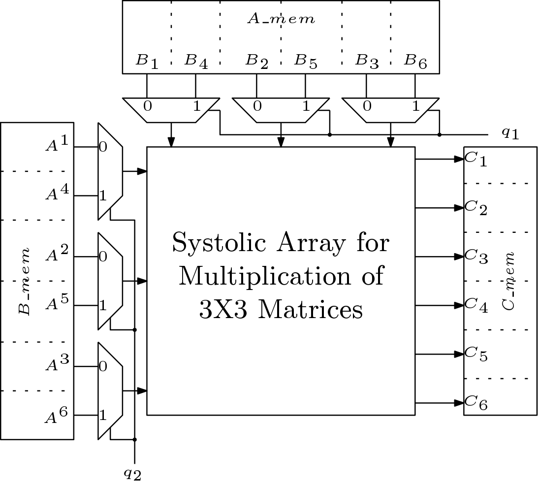
Here matrix A (6X6) and matrix B (6×6) are multiplied together and the result is matrix C (6×6). The matrix A and matrix B are stored in memory banks and respectively. These memory banks have six memory elements. Each element can be configured as ROM or RAM. The columns of matrix B and rows of matrix A can accessed serially. Here denotes row of matrix A and denotes column of matrix B.

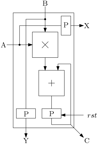
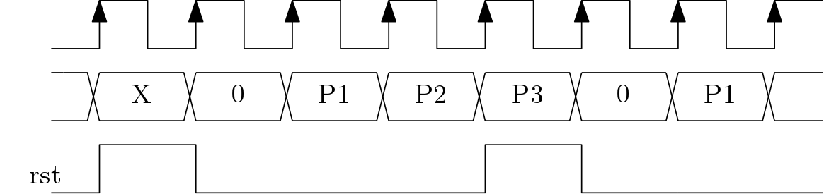
We will first discuss the systolic matrix multiplier for 3×3 matrices and then we will use the systolic architecture for 3×3 matrix to design a multiplier for 6×6 matrices. Here, the basic data processing unit is called as Multiply-Acumulate unit (MAC). The architecture of the MAC is shown in Figure 1. The MAC block implements the function . It has a reset input to start new accumulation. The timing diagram for the MAC block is shown in Figure 2 with reset input.

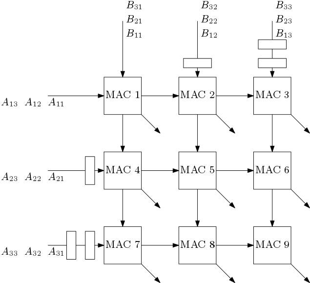
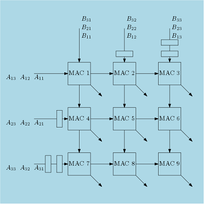
The overall systolic architecture to multiply 3×3 matrices is shown in Figure 3. Here, six MAC blocks are used. In this architecture, from one side the rows of A and from another side columns of B are fed. The 2nd row of A and 2nd column of B are delayed by one clock cycle. This is because, we want to compute one element of matrix C per cycle. Similarly two clock delay are applied to the 3rd row of A and 3rd column of B.

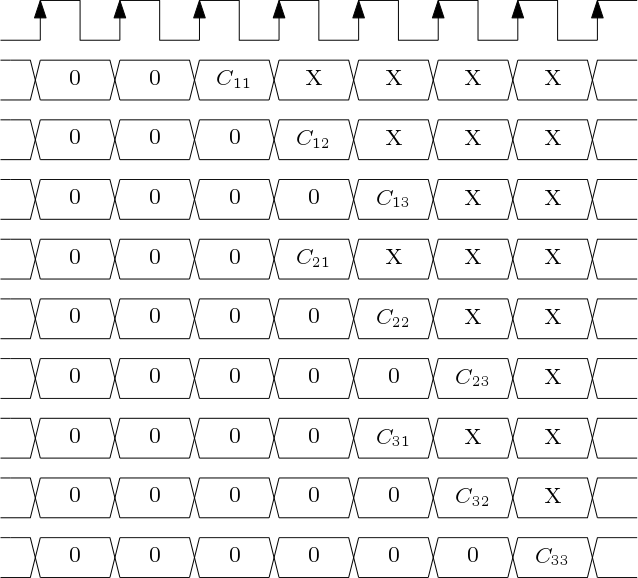
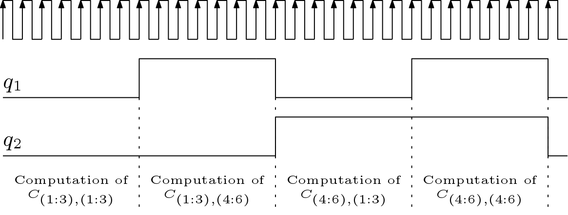
The timing diagram for computation the above mentioned architecture is shown in Figure 4.

The above mentioned systolic architecture to multiply 3×3 matrices can be used to multiply two 6×6 matrices. The systolic matrix multiplier for 6X6 matrices is shown in Figure 5. The columns of B and rows of A are fed to the systolic array through MUXes. In the first phase, first three rows of A and the first three columns of B are multiplied. In the second phase, first three rows of A are multiplied with last three columns of matrix B. The phase wise computation of C is shown in Figure 6.

Timing Complexity: The multiplication of two 6X6 matrices is accomplished in four phases. Thus first part of timing complexity is (4X6 = 24 clock cycles). In the mean time, the reset signal is asserted three times. Thus three clock cycles are elapsed for clearing. The architecture is systolic and thus extra four clock cycles are needed. Total clock cycles are

 clock cycles.

This architecture is better than the vector-vector multiplication based architecture in terms of speed for the similar hardware. But for higher matrix size, this architecture may not be suitable.

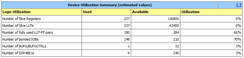
Hardware Utilization: The FPGA performance of this architecture is shown below. Here, total 6 MAC blocks are used. Each MAC has one multiplier and one adder. Total 6 MUXes are used.