Vector-Vector Multiplication - Digital System Design

Apart from scalar-vector multiplication, Vector-Vector multiplication is another very important arithmetic operation in implementing signal or image processing algorithms. The matrix multiplications can also be achieved through vector-vector multiplication which is also called as inner product computation.

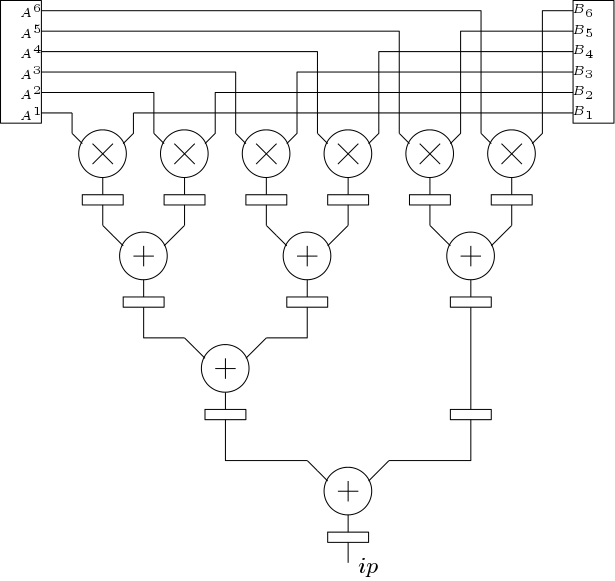
In this tutorial, we will discuss multiplication of matrix A (6X6) with matrix B (6X6) using Vector-Vector multiplication. The multiplication result is matrix C (6X6). The Vector-Vector multiplier is shown in Figure 1. Here, matrix A is shown in a memory bank and B matrix is also stored in another memory bank. These memory banks can be configured as ROM or RAM. The memory banks has six outputs and each output is a word. Here, $A^i$ denotes $i^{th}$ row of matrix A and $B_i$ denotes the $i^{th}$ column of matrix B.

The first stage of the Vector-vector multiplier is multiplier stage and the second stage is adder tree. If there are n elements in the vector, then there will be n multipliers used and (n-1) adders will be needed in the adder tree. The pipeline registers are inserted between adders or between a multiplier and an adder.

Timing Complexity: The total timing complexity to multiply two 6×6 matrices is expressed as

$T = T_{lat} + n^2$

Here, $T_{lat}$ is the latency period of the Vector-vector multiplier and it is equal to four clock cycles. The second term is for multiplying two nxn matrices. Thus total time taken to multiply two 6X6 matrices is (4 + 36=40) clock cycles. After the latency period, we get one inner product per cycle. Then these outputs can be written to any other memory blocks.

Related Posts