Signal processing algorithms sometimes involve computation of exponential. Thus it is important to implement the exponential function. In this work, design of digital hardware for exponential function is discussed. Like other elementary functions, exponential function is also computed using the iterative formulas. In this work, computation of the exponential function  is shown for three cases.
- When
 is positive.
 - When is negative.
- When is positive or negative.
1. Computation of when is Positive
The computation of is governed by the following two equations.
(1) 
where  varies from
  to
to  which is the total number of iterations. Initially,
  and
and  . A new parameter
  is defined to find the values of
  . It is computed as
  .
.
(2) 
When  the equations (1) is modified as
(3) 
and when  the equation (1) becomes
(4) 
After iterations the final values of  and
and  are
are
(5) 
In other way, the following equation is also true
(6) 
Implementation of Exponential Function for Positive Values
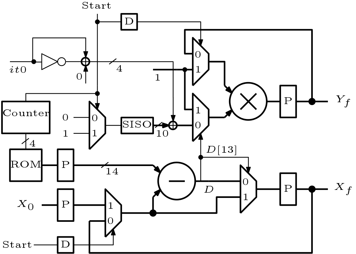
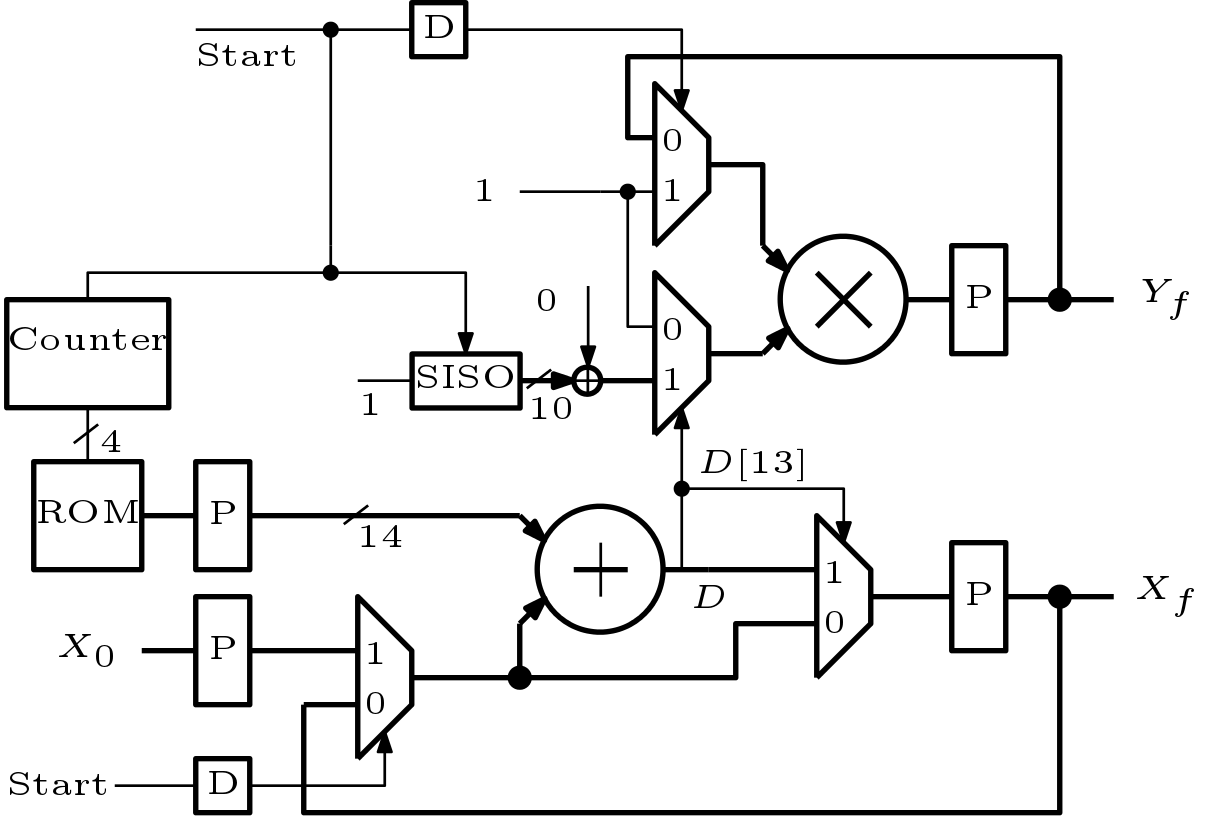
Based on the above equations, a serial architecture is developed in this work to compute when is positive. The architecture is shown in Figure 1. The minimum data-width which is required in this architecture is 14 to support all the results. Out of 14-bits, 10-bits are used for fractional part. Total 11 iterations are required. The values of  for 10-bit precision is shown in Table 1. These values are stored in ROM and size of it is
  . Initially a
  signal loads in a register and starts the counter. The delayed version of signal chooses initial value ‘1’ for the multiplier and also chooses as initial value to the subtracter. A Serial Input Serial Output (SISO) is used to generate the values of
  . The symbol
  in Figure 1 indicates concatenation operation. This operation take place like the following way

Where  signal indicates iteration zero or first iteration. Computation of next data is started by clearing the final values of
  and
and  . The new value of is again stored in the register. At least 12 clock cycles are required in computation of one exponential function.
 when is positive.
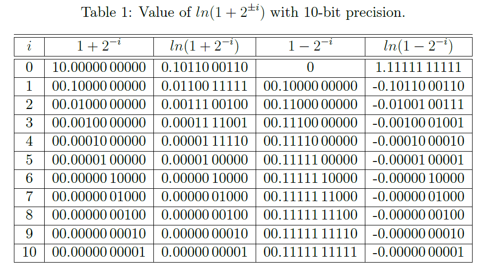
2. Computation of when is Negative
The computation of when is negative is done in the same way as it was computed in the previous section. The parameter is computed as  .
.
(7) 
When the equations (1) is modified as
(8) 
The equation (1) when is same for both the cases. The final equations are also same.
The range of is is controlled by the following equation
(9) 
thus the range of is  .
.
Implementation of Exponential Function for Negative Values
Architecture to compute when is negative is very similar to the architecture discussed previously. The architecture is shown in Figure 2. Here ROM stores the values of  as shown in Table 1. The size of the ROM is 1-bit higher than the ROM which was previously used to store
  . In place of subtracter, an adder is used here. The concatenation operation take place like the following way

In order to compute the exponential of next value of , the values of and must be cleared. The SISO is also needed to cleared.
 when is negative.
 3. Computation of when can be +ve or -ve
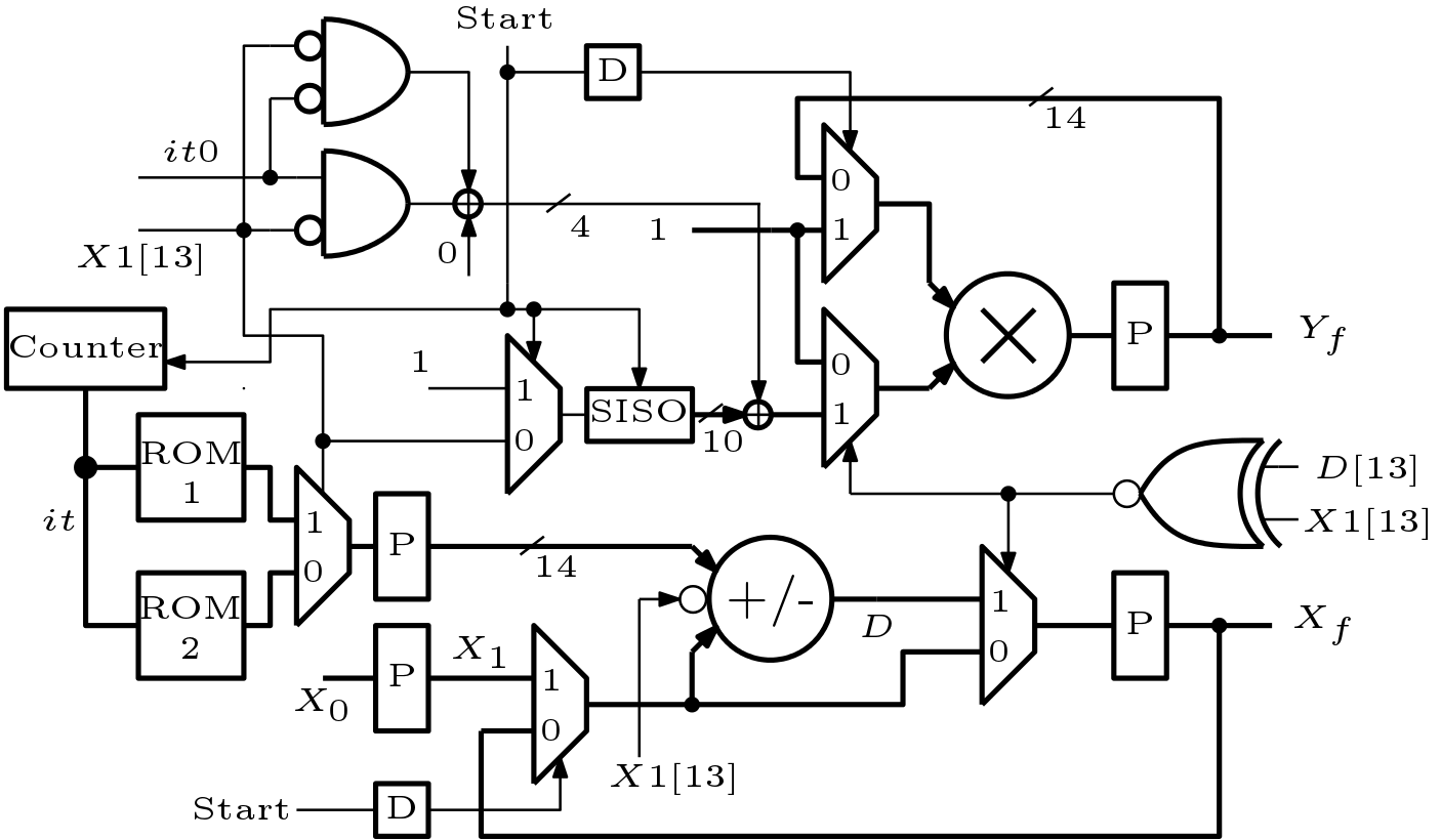
It is important to compute by a same hardware when can be both positive or negative. Thus Figure 1 and Figure 2 is combined and a new architecture is developed which is shown in Figure 3. Two ROMs are used here. ROM 1 stores values of and ROM 2 stores values of . If is negative then data is read from ROM 1. An adder/subtracter is used here which is controlled by invert of the MSB of  .
.
 when can be both positive or negative.
Conclusion
Computation of exponential function can be done by other methods also like CORDIC but this method is more accurate than the CORDIC based method. The range of exponential function can be increased by scaling of input data and by including a post scalar block.