Singular Value Decomposition (SVD) is one of the matrix factorization techniques which can be used to solve linear equations. But this is not the primary objective of SVD. SVD can provide singular values of matrix. Singular values reveal unique information about a matrix. SVD has many uses in machine learning, image processing etc. Linear equations also can be solved using SVD. Objective of this tutorial is to discuss strategies for implementation of SVD which can help a reader to understand how hardware architectures can be developed for SVD. Detailed theoretical background is beyond the scope of this tutorial.
SVD is a matrix factorization technique which factors a matrix (A) into three different matrices as shown below

Here, A is the input matrix, U is an orthogonal matrix, S is a matrix in which all the elements above or below the diagonal are zero, and V is another orthogonal matrix. Diagonal elements of S are the singular values of A. In most cases, our primary objective is to obtain the S matrix. Obtaining U and V matrix is not required. There are three algorithms by which SVD can be obtained. They are Golub-Kahan Algorithm, Divide and Conquer Algorithm, and Jacobi Algorithm. Jacobi Algorithm is the most popular algorithm to implement SVD. In this tutorial we will discuss, Jacobi Algorithm for implementing SVD. There are two type of Jacobi algorithm for obtaining SVD. They are Jacobi-Kogbetliznt algorithm or double-sided Jacobi method and Jacobi-Hestenes algorithm or single-sided Jacobi algorithm.
Implementation of SVD using Double Sided Jacobi Method
The main principle of the Jacobi method is that matrix A is multiplied by Jacobi Rotation matrices successively to nullify the off-diagonal elements. Multiplication is done from both left and right sides of matrix A. Left side Jacobi matrices are denoted as  and right-side Jacobi matrices are denoted as
  . Multiplication by the Jacobi matrices is shown below.

Here,  represents the number of iterations after which we get the singular values. The orthogonal matrices can be computed as
 ,
, 
This method is called double sided as matrix A is multiplied by Jacobi rotation matrices from both sides. Multiplication by left Jacobi matrix means rotation of rows of A and multiplication by right Jacobi matrix means rotation of columns of matrix A. The process of double-sided Jacobi method for SVD is shown in Figure 1 for a 4×4 matrix.
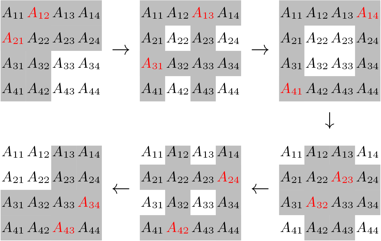
In the above figure, the elements which are to be nullified are shown by color Red. Gray color indicates the Rows and Columns which will be modified in nullifying a Red colored element. Above process is called as a sweep. Here, in a sweep we are trying to nullify 12 elements. In one iteration of a sweep two elements are nullified and there are 6 iterations in a sweep. One sweep is not enough to make all the off-diagonal elements zero. Many sweeps may be required to obtain singular values, but it depends on some criteria based on error. A MATLAB code is shown below for this technique which includes all the necessary equations also.
function [U,S,V] = JOS_SVD1(G,U,V,it)
P = zeros(2,2);
n = size(G, 2);
 S = eye(n);
    for k =1:it
    for i = 1:n-1%%% 1 to 2
        for j = i+1:n %%%%2 to 3
        P(1,1)=G(i,i);
        P(1,2)=G(i,j);
        P(2,1)=G(j,i);
        P(2,2)=G(j,j);
        theta=0.5*(atan((P(2,1)+P(1,2))/(P(2,2)-P(1,1))) - atan((P(2,1)-P(1,2))/(P(2,2)+P(1,1))));
        phi=0.5*(atan((P(2,1)+P(1,2))/(P(2,2)-P(1,1))) + atan((P(2,1)-P(1,2))/(P(2,2)+P(1,1))));

            cs = cos(theta);%%not required if CORDIC is used.
            sn = sin(theta);%%not required if CORDIC is used.
            cs1 = cos(phi);%%not required if CORDIC is used.
            sn1 = sin(phi);%%not required if CORDIC is used.
            x = G(i,:);
            G(i,:) = cs*x - sn*G(j,:);
            G(j,:) = sn*x + cs*G(j,:);

            % update U
            x = U(i,:);
            U(i,:) = cs*x - sn*U(j,:);
            U(j,:) = sn*x + cs*U(j,:);

            % update G
            x = G(:,i);
            G(:,i) = cs1*x - sn1*G(:,j);
            G(:,j) = sn1*x + cs1*G(:,j);

            % update V
            x = V(:,i);
            V(:,i) = cs1*x - sn1*V(:,j);
            V(:,j) = sn1*x + cs1*V(:,j);
        end
    end
    end

for i = 1:n
    S(i,i) = G(i,i);
end
Double Sided Jacobi Method with CORDIC
Multiplication of Jacobi matrices means either column wise rotation or row wise rotation and we know that rotation can be achieved by CORDIC algorithm. Two CORDIC rotations are required in an iteration of a sweep, one row wise and one column wise. The U and V matrices also can be achieved with CORDIC based SVD strategy. This CORDIC based implementation of SVD is shown in Figure 2.
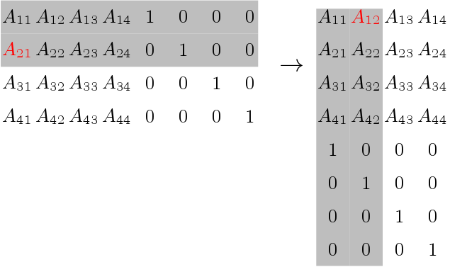
Here, Identity matrices are also sent along with matrix A to CORDIC block to obtain matrix U and V. If U and V matrices are not required, then it is no required to send the identity matrices. The MATLAB function for CORDIC based SVD is shown below.
function [U,G,V] = JOS_SVD_CORDIC(G,U,V,it)
P = zeros(2,2);
n = size(G, 2);
 S = eye(n);
    for k =1:it
    for i = 1:n-1%%% 1 to 2
        for j = i+1:n %%%%2 to 3
        P(1,1)=G(i,i);
        P(1,2)=G(i,j);
        P(2,1)=G(j,i);
        P(2,2)=G(j,j);
        theta(i,j)=0.5*(atan((P(2,1)+P(1,2))/(P(2,2)-P(1,1))) - atan((P(2,1)-P(1,2))/(P(2,2)+P(1,1))));
        phi(i,j)=0.5*(atan((P(2,1)+P(1,2))/(P(2,2)-P(1,1))) + atan((P(2,1)-P(1,2))/(P(2,2)+P(1,1))));
        alpha = theta(i,j) ;
        beta = phi(i,j) ;

            for k = 1:n
            [G(i,k),G(j,k),z1] = cordic_rotation(G(i,k),G(j,k),alpha);
            end

            for k = 1:n
            [U(i,k),U(j,k),z2] = cordic_rotation(U(i,k),U(j,k),alpha);
            end

            for k = 1:n
            [G(k,i),G(k,j),z3] = cordic_rotation(G(k,i),G(k,j),beta);
            end

            for k = 1:n
            [V(k,i),V(k,j),z4] = cordic_rotation(V(k,i),V(k,j),beta);
            end
        end
    end
    end

for i = 1:n
    S(i,i) = G(i,i);
end
MATLAB function to achieve CORDIC rotation is given below.
function [x1,y1,z1] = cordic_rotation(x,y,z)
 k = 20;
 z1 = (z);
 kn = 0.6073;

for idx = 0:k
    xtmp = bitsra(x, idx); % multiply by 2^(-idx)
    ytmp = bitsra(y, idx); % multiply by 2^(-idx)
    ztmp = atan(2^(-idx));
    if z1 > 0
        x(:) = x - ytmp;
        y(:) = y + xtmp;
        z1(:) = z1 - ztmp;

    else
        x(:) = x + ytmp ;
        y(:) = y - xtmp;
        z1(:) = z1 + ztmp;
    end

end
x1 =  x*kn;
y1 =  y*kn;
end
The main MATLAB code to run the double sided SVD is given below.
clear all;
close all;
 A = [1,2,3,4;2,3,4,5;3,4,5,6;4,5,9,7];
 n = size(A,2);
 it = ceil(log2(n)) + 1;
 n = size(A,2);
 U1 = eye(n);V1 = eye(n);
 [U2,S1,V2] = JOS_SVD1(A,U1,V1,it);
 A3 = V2*S1*U2;

 [U3,S2,V3] = JOS_SVD_CORDIC(A,U1,V1,it);
 A4 = V3*S2*U3;

 S3 = svd(A);
Implementation of SVD using Single Sided Jacobi Method
Double sided Jacobi technique needs rotations from both sides. This requirement makes this algorithm difficult for parallelism. Double sided Jacobi algorithm is very fast in serial architectures. Jacobi and Hestense together came up with another algorithm for implementation of SVD which is known as single sided Jacobi method. Here, multiplication from one side is enough. This method is based on the idea that.

This equation is obtained by multiplying both side of the original SVD equation by V. In this technique, we bother to calculate  matrix. Then other two matrices S and U can be obtained using matrix B. The mathematical equations and the strategy are shown in the MATLAB code for single sided Jacobi method.
clear all;
close all;
A1 = randn(32,32);
[M,N] = size(A1);
A = A1;
for it = 1:8
for i = 1:N-1
    for j = i+1:N
Q = A(:,i)'*A(:,i) - A(:,j)'*A(:,j);
P = 2*A(:,i)'*A(:,j);
V = sqrt(P^2 + Q^2);

if Q >= 0
c = sqrt((V+Q)/(2*V));
s = P/sqrt(2*V*(V+Q));
else
s = sqrt((V-Q)/(2*V));
c = P/sqrt(2*V*(V-Q));
end
B = [A(:,i),A(:,j)]*[c,-s;s,c];
A(:,i) = B(:,1);
A(:,j) = B(:,2);
    end
end
end
for i = 1:N-1
    for j = i+1:N
        nul(i,j) = A(:,i)'*A(:,j);
    end
end
F = A'*A;
S1 = diag(real(sqrt(A'*A)));

result = [svd(A1),S1]%%%Match the values with S1...............
User can choose any one algorithm for implementation of SVD. SVD is not suitable for solving linear equations. Thus, evaluating only the S matrix is enough. There is no need to evaluate the U and V matrices. Double sided Jacobi method is suitable for Serial architectures and single sided Jacobi is suitable if the original algorithm involves many vector-vector multiplication. CORDIC implementation involves errors and high latency.