Fast Computation of Square Root and its Reciprocal

Bhakshali Algorithm

This method for finding an approximation to a square root or square root reciprocal was described in an ancient Indian mathematical manuscript. This algorithm is quartically convergent. The iterative equations are

$a_i = \frac{(X-x^2_{i-1})}{2x_{i-1}}$

$b_i = a_i + x_{i-1}$

$x_i = b_i - \frac{a^2_{i}}{2b_i}$

The variable $a_n$ approaches zero and $x_n$ holds the value of square root.

Two variable iterative method

This method is used to find square root of number 1<X<3. However the range of $X$ can be increased. This method converges quadratically. The equations are

$a_i = a_{i-1} - 0.5\times c^2_{i-1}$

$c_i = 0.5c^2_i(c_{i-1} - 3)$

Initially $a_0 = X$ and $c_0 = X-1$ . Finally the variable $a_n$ holds the final value of $\sqrt{X}$ .

Halley’s method

Halley’s method is actually the Householder’s method of order two. The equation which governs this algorithm is

$y_i = X\times x^2_{i-1}$

$x_i = \frac{x_{i-1}}{8}(15 - y_i (10 - 3 y_i))$

At the final step, $x_n$ holds the value of square root reciprocal of $x$ and $y_n$ converges to 1. This method converges cubically but involves four multiplications per iteration.

Newton Raphson Iteration

Newton-Raphson’s iterative algorithm is a very popular method to approximate a given function. It can be used to compute square root or square root reciprocal of a given number. The Newton-Raphson’s iterative equation is

$x_{i+1} = x_i - \frac{f(x_i)}{{f_1}(x_i)}$

where $f_1(x_i)$ is the derivative of $f(X_i)$ . The function which is used to compute the square root reciprocal of a number is $f(x) = (1/x^2) - X$ , where X is the input operand. The Newton-Raphson iteration gives

$x_{i} = 0.5\times x_{i-1}(3 - X\times x^2_{i-1})$

Here $x_0$ is taken as close approximation of $\frac{1}{\sqrt{X}}$ . After some finite iterations the above equation converges to the square root reciprocal of X. It is very obvious that the value of $x_0$ must be chosen care fully to converge.

The square root of $X$ can be computed by multiplying the final output $x_n$ by $X$ or directly iterating for square root. The function $f(x) = (x^2) - X$ can be used in this case. Then the iterative equation will be

$x_{i} = 0.5\times(x_{i-1} + \frac{X}{x_{i-1}})$

Similar to the previous algorithms here also $x_0$ takes the closest approximation of $\sqrt{X}$ . One of the disadvantage of direct computation of square root by Newton’s theorem is that it involves a division operation which is much complex than a multiplication operation.

Gold-Schmidt Algorithm

The Gold-Schmidt algorithm is one of the popular fast iterative methods. This algorithm can be used to compute division, square root or square root reciprocal. The basic version of the Gold-Schmidt algorithm to compute square root reciprocal of the radicand X is governed by the following equations. All these equations are sequentially executed in a iteration.

$b_i = b_{i-1}\times Y^2_{i-1}$

$Y_i = (3 - b_i)/2$

$y_i = y_{i-1} \times Y_i$

Initially $b_0 = X$ , $Y_0$ = a rough estimate of $\frac{1} {\sqrt{X}}$ and $y_0 = Y_0$ . The initial guess of $Y_0$ can be done by selecting a close value from a predefined LUT. The algorithm runs until $b_i$ converges to 1 or for a fixed number of iterations. Finally square root reciprocal is computed as, $y_n = \frac{1}{\sqrt{X}}$ . Note that this algorithm can be used to compute both square root and its reciprocal. The square root function can be computed by multiplying the final value of $y$ by $X$ as $x_n = X\times y_n$ . This algorithm involves three multiplications and one subtraction per iteration to compute $y_n$ . Square root can be computed by another multiplication at the end.

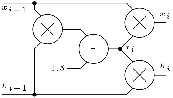
Another version of Gold-Schmidt algorithm is shown below

$r_i = 1.5 - x_{i-1}\times h_{i-1}$

$x_i = x_{i-1}\times r_i$

$h_i = h_{i-1}\times r_i$

Here initially $y_{0}$ equals to the closest approximation of the function $\frac{1}{\sqrt{X}}$ , $x_0 = X\times y_0$ and $h_0 = 0.5y_0$ . At the end of the iterations $x_n$ converges to $\sqrt{X}$ and $2h_n$ converges to $\frac{1}{\sqrt{X}}$ . This algorithms runs until $r_i$ reaches close to 0 or for fixed number of iterations. This improved version of Gold-Schmidt algorithm is faster than its previous version as at output stage no multiplier is needed to compute the square root function. But number of arithmetic operations per iteration remains same.

Choice of Algorithm

The algorithms discussed above computes square root and its reciprocal by sequential execution of some equations until stopping criteria is reached or for a fixed number of iterations. In software application, the choice of algorithm is not so crucial but in hardware implementation the algorithm must be chosen carefully. Following are the criteria to select an algorithm.

Resources: Implementation of the algorithm must be hardware efficient. (Number of multiplication and addition per iteration)
Iteration Count: Iterative algorithms mentioned above are meant to be faster, so the chosen method should produce an acceptable estimate after minimum number of iterations.
Error: The acceptable amount of error is an important metric in choosing an algorithm.
Initial Guess: Technique to choose the initial value should be simple otherwise extra storage is wasted.

Two methods among the above mentioned algorithms, Newton-Raphson and Gold-Schmidt Algorithm are popularly used. In this tutorial, we have chosen the Gold-Schmidt Algorithm (version 2) for implementation. The implementation of Gold-Schmidt Algorithm is discussed below.

Related Posts