Pipeline Implementation of IIR Low Pass Filter

Majority of digital filters implemented in the digital systems are Finite Impulse Response (FIR) filters. Infinite Impulse Response (IIR) filters can produce same frequency response but with less co-efficients and delay elements compared to FIR filters. But use of IIR filters is limited to the low frequency applications. This is due to the fact that IIR filters have longer critical path due to their recursive nature. In this work, various parallel structures of IIR filters are implemented on Field Programmable Gate Array (FPGA) device. Also, pipeline implementation of IIR filters is investigated. All these implementations are implemented by taking an example of low pass filter. FPGA implementation performance of all the structures are compared. Root Mean Squared Error (RMSE) is used to estimate the performance.

I. IIR Low Pass Filter

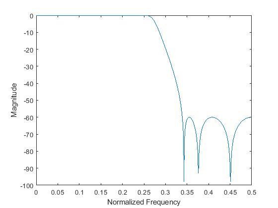
In this work, design of a low pass filter is taken as an example to illustrate the implementation of IIR filter. The frequency response of the low pass filter is specified as

$\begin{cases} \alpha_p = 0.01\hspace{1pt}dB & \text{for}\hspace{2pt} 0\leq w \leq \frac{\pi}{3}\\ \alpha_s = 60\hspace{1pt}dB & \text{for}\hspace{2pt} \frac{\pi}{3}\leq w \leq \frac{\pi}{2} \end{cases}$

Here, w is the normalized frequency. The parameter $\alpha_p$ and the $\alpha_s$ denotes the pass band and stop band attenuation. This low pass IIR filter can be realized using many techniques. Here elliptical based design is followed. The transfer function of an IIR filter can be written as

Here, N=M=6 for the given low pass filter. The frequency plot of the low pass IIR filter is shown in Figure 1.

Figure 1: Frequency plot for the IIR LPF

IIR Filter Matlab Code (2194 downloads )

II. Different IIR Filter Structures

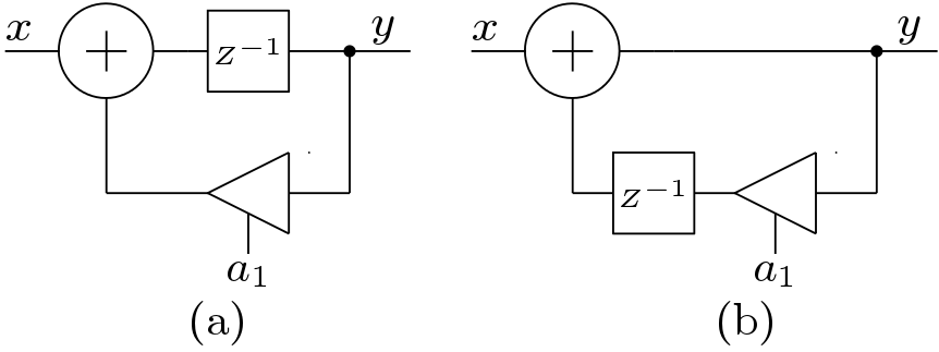
A. Direct Form I

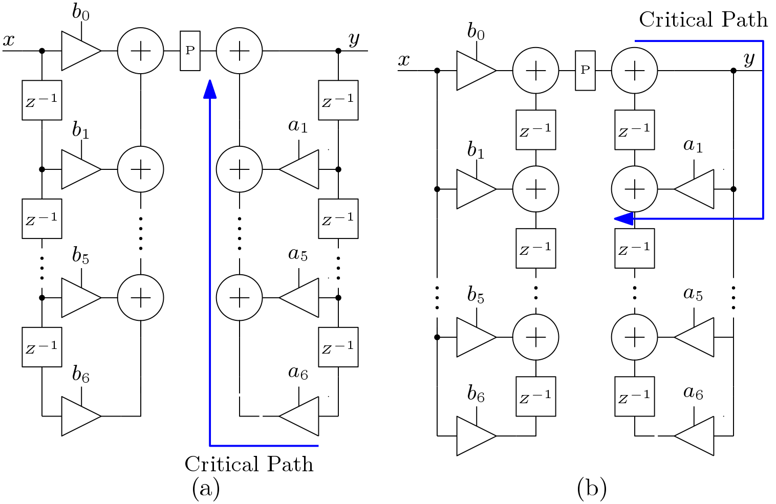
The direct form I structures directly implements the IIR filters. The basic direct form I structure is shown in Figure 2(a). The implementation of this kind of architecture is not suitable for implementation as this structure has very high critical path in the all pole transfer function section or in the recursive section. If the pipeline registers are added, the result will be changed as inclusion of extra registers will implement a different filter. An alternative direct form I architecture is shown in Figure 2(b) which is called transposed direct form I structure. Here the critical path is reduced.

B. Direct Form II

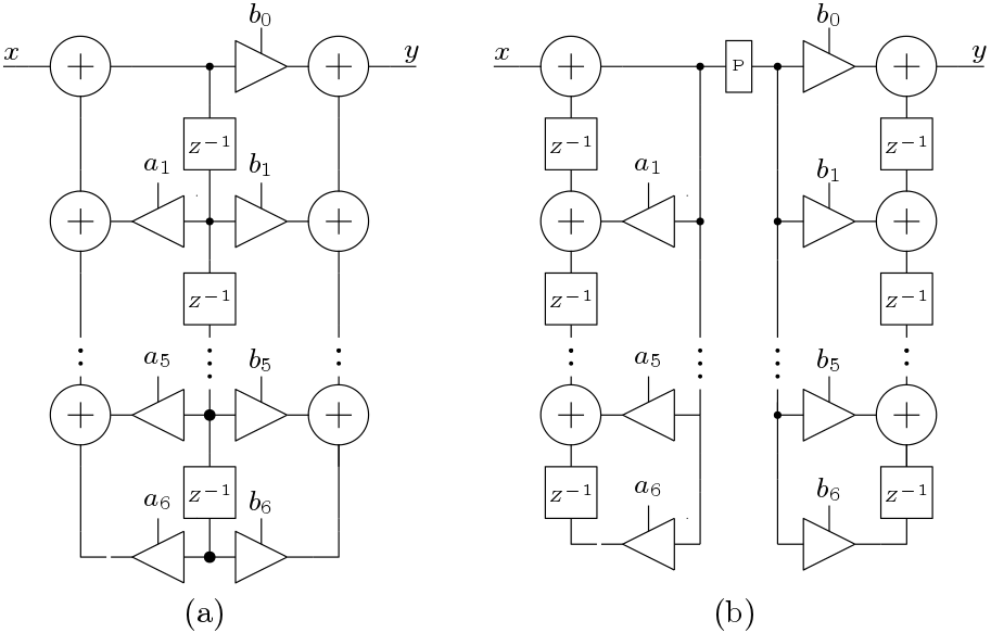
The basic direct form II structure is shown in Figure 3(a). This structure uses less number of delay elements compared to the direct form II structure but has the same critical path. But this structure is also not suitable for the high frequency applications. The transposed architecture is shown in Figure 3(b). This architecture reduces the critical path. All though transposed structures for direct form I and direct form II are same, direct form II structures are not preferred. In direct form II structures, a high gain all pole network is followed by a all zero network. This increases the size of the adders and multipliers.

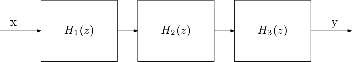
C. Cascaded Structure

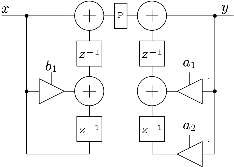
Here, H(z) can be written in terms of smaller transfer functions. These smaller transfer functions can be 1st order IIR transfer function or second order IIR transfer function. The second order IIR section is popularly known as Biquad structure. The Biquad transfer function is

$H(z) = \frac{\sum^{M}_{n=0}b_nz^{-n}}{1 - \sum^{N}_{n=1}a_nz^{-n} }$

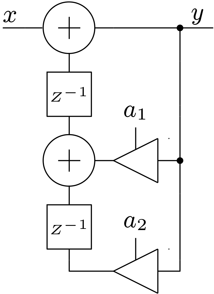
Biquad structure is shown in the Figure 4 and the cascaded form of the IIR LPF is shown in Figure 5.

Figure 4: Biquad Structure for IIR Cascaded Form

Figure 5: Cascaded Form of the IIR LPF Filter

D. Parallel Structure

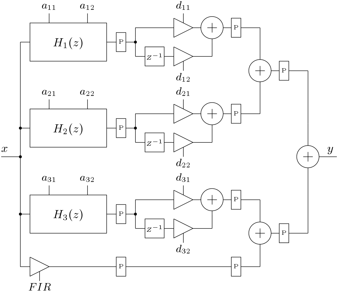
The parallel forms of IIR filters gained more popularity than the cascaded forms as parallel forms provide immunity to the co-efficient quantization and also provide parallelism in the design. In the parallel form, the IIR transfer function is written as summation of 1st order or second order sections. This is usually achieved using the partial fraction procedure. Generally Biquad structures are preferred as individual sections. The IIR low pass filter transfer function considered here can be written as

$H(z) = FIR + \sum_{i=1}^L \frac{d_{i1} + d_{i2}z^{-1}}{1 - a_{i1}z^{-1}-a_{i2}z^{-2}}}$

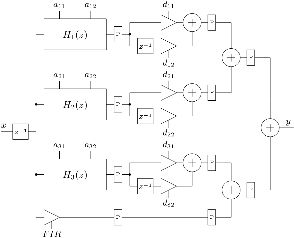
Here the FIR is a simple constant and L denotes the number of parallel sections. The above equation is for non-delayed architecture. The delayed input signal is some times provided to the all pole section when the order of numerator is greater than the order of denominator. This form is known as delayed parallel structure. In this case, FIR part can be a FIR like transfer function. The second order section for the parallel structure of the low pass filter considered here is shown in Figure 6. The non-delayed and delayed parallel structure is shown in Figure 7 and 8 respectively.

Figure 6: Biquad Structure for Parallel Architecture

Figure 7: Non-delayed Parallel IIR LPF Structure

Figure 7: Delayed Parallel IIR LPF Structure

III. Pipeline Implementation of IIR Filters

The direct form structures are not generally suitable for high frequency applications due to their long critical path. The transposed architectures remove this drawback of the direct forms. The longer critical path is still a concern. Insertion of pipeline registers is not possible as it will implement any other filter. Thus special algorithms are reported to implement pipeline IIR filters. Let’s consider the case of a simple 1st order filter. The transfer function of the 1st order filter is

$H(z) = \frac{1}{1 - az^{-1}}$

This filter can be implemented in two ways. One is direct form and another is transposed form. These structures are shown in Figure 9. In both the cases, the maximum frequency is limited by the combinational delay of an adder and a multiplier. This delay can not be reduced by inserting pipeline registers.

IIR Low pass filter — Figure 9: Different Structure of !st order filter.

The Look-ahead pipelining techniques are very popular to insert pipeline registers in the IIR filters. The original transfer function has a single pole at z=a. The P-stage pipeline implementation is derived by adding (P-1) poles and zeros at identical locations. The pipeline implementation of the 1st order filter is derived by the following equation

$H(z) =\frac{\prod_{i=0}^{log_2^{P-1}}(1 + a^{2^i}z^{-2^i})}{1 - a^Pz^{-P}}$

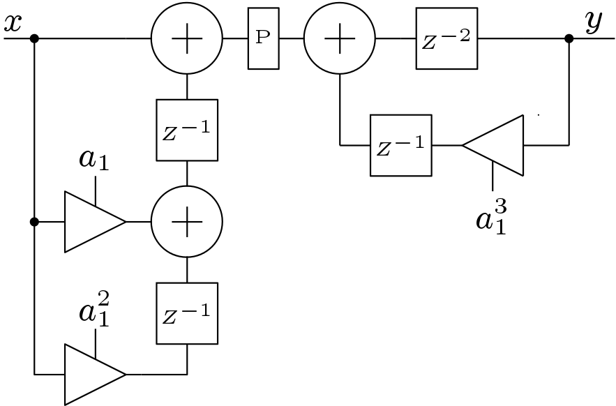
The transfer function for the three stage pipeline implementation of the 1st order filter is shown below

$H(z) = \frac{1+az^{-1}+a^2z^{-2}}{1 - a^3z^{-3}}$

The pipeline structure of the 1st order IIR filter is shown in Figure 10. Here, the critical path is obviously reduced by atleast three times. Thus this circuit can be operated at high frequencies. But the hardware complexity of the implementation increases.

Figure 10: Pipeline Implementation of the 1st order IIR filter

There exists two Look-ahead techniques to implement pipeline IIR filters which are

Clustered Look-ahead Technique
Scattered Look-ahead Technique

In both the techniques, pipeline implementation of 1st order IIR filter is same. A P stage pipeline implementation using the Clustered Look-ahead technique for the higher filter is obtained by multiplying the numerator and denominator by

$\sum_{i=0}^{P-1}r_iz^{-i}$

where  is evaluated as follows

$\begin{cases} r_{-1}=0 & for\hspace{2pt} i=0,1,2,....,(N-1)\\ r_{i}=0 & for\hspace{2pt} i=0\\ r_{i}=\sum_{k=1}^{N}a_kr_{i-k} & i>0 \end{cases}$

Here (P-1) additional canceling poles and zeros are inserted. This method suffers from the stability problem. The pipeline implementation obtained from this method can be unstable even though the original transfer function was stable. Stable implementation can be obtained by inserting higher pipeline stages.

Other technique to obtain pipeline implementation is scattered Look-ahead technique. Lets, consider the denominator of a transfer function is represented as

$D(z) = \prod_{i=1}^P (1 - p_iz^{-1})$

Then the P-stage pipeline implementation in this technique is obtained by the following equation

$H(z) = \frac{N(z)}{D(z)} = \frac{N(z)\prod_{i=1}^N \prod_{k=1}^{P-1}{(1 - p_ie^{j2\pi k/P}z^{-1})}}{\prod_{i=1}^N \prod_{k=0}^{P-1}{(1 - p_ie^{j2\pi k/P}z^{-1})}}$

This technique guarantees stability with less number of pipeline stages in comparison to the clustered Look-ahead technique. Both the techniques implements pipeline IIR filters with increased hardware complexity. It is better to apply this technique to the second order transfer functions instead of applying directly to the main transfer function. The second order transfer function $H(z) = 1/(1 - a_1z^{-1} -a_2z^{-2})$ is transformed into the following transfer function

$H(z) = \frac{1 + a_1z^{-1} + (a^2_1 + a_2)z^{-2} - a_1a_2z^{-3} + a^2_2z^{-4}}{1 - (a^3_1 + a_1a_2)z^{-3} - a^3_2z^{-6}}$

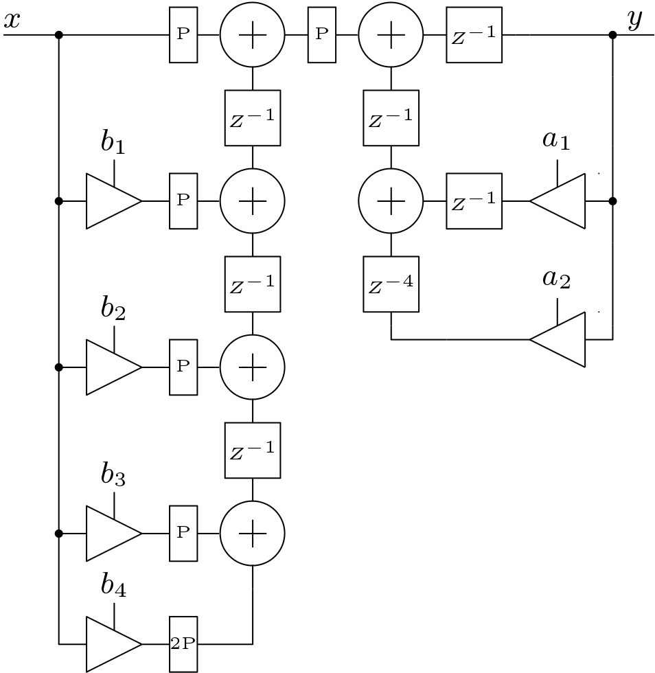
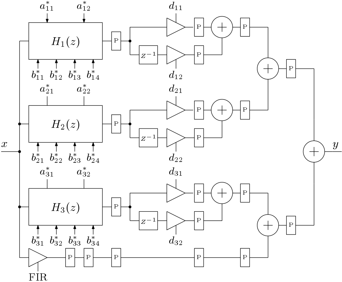
In this work, pipeline implementation of the IIR low pass filter is presented. The parallel IIR low pass filter is chosen here for pipeline implementation. The scattered Look-ahead technique is applied to the second order Biquads. The modified Biquad structure is shown in Figure 11. The resulting pipeline parallel IIR low pass filter is shown in Figure 12. Here the star marked co-efficients are the co-efficients of pipelined version of the IIR filter.

IV. Performance Estimation

A. Design Performance

In this work, low pass IIR filter of order 6 is implemented on NEXYS DDR2 artix7 FPGA device (xc7a100t-3csg324). The low pass filter is verified by taking two sinusoidal signals of frequencies 22 KHz and 20 KHz. These two signals are multiplied and output of the multiplier is given to the low pass filter. The sampling frequency is taken as 100 KHz and thus the low pass filter filters out the signals whose frequency greater than 25 KHz. The output of the filter is a tone of 2 KHz which is shown in Figure 13. The original output signal obtained from MATLAB and the FPGA based filtered output (delayed version) is compared in Figure 13.

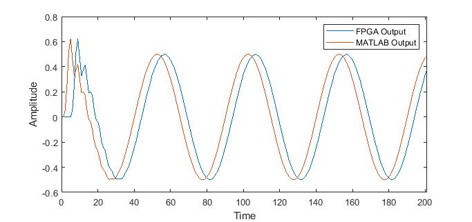
Figure 13: Comparison of IIR filter output at Matlab vs output of FPGA

Here, 18-bit fixed point data width is chosen for implementation where 10-bit is reserved for fractional part. Here, Root Mean Squared Error (RMSE) is used to measure the design performance. RMSE is computed as

$RMSE = \frac{{\left\lVert(\hat{y}-y)\right\rVert}_2}{{\left\lVert y \right\rVert}_2}$

Here y is MATLAB based filtered output and $\hat{y}$ is FPGA output. A RMSE of 0.0059 is achieved using 18-bits of word length for parallel IIR implementation. A RMSE of 0.00584 is achieved when the same parallel filter is implemented for higher frequency application.

B. Comparison of Different IIR Filter Structures

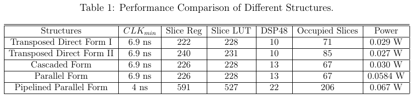
The performance of the FPGA implementation of different IIR low pass filter structures are compared and this comparison is shown in Table 1. The performance of the transposed direct form structures are almost same. The cascaded structures are preferred over direct forms due to its immunity towards the quantization noise. The cascaded structures consume slightly higher resources and have higher latency. The parallel structures are more popular than any other structures. They have similar immunity towards the quantization noise and also introduces parallelism to the design. Thus latency is reduced but consumes more hardware than direct forms. All these structures are not suitable for higher frequency applications as they have longer critical path. This critical path is due to the delay of two adders and one multiplier. This critical path is reduced in the pipelined parallel IIR filter. Higher maximum frequency is achieved with the cost of extra hardware.

V. Conclusion

In this work, FPGA implementation of the different IIR filter structures is presented and a comparison of the performances is presented here. Here, a low pass filter is designed using different structures to demonstrate difference in implementation. Transposed direct form structures are very popular as they have shorter critical path. In fixed point implementation, cascaded and parallel structures provide less quantization noise compared to the direct forms. All this structures suffer from the long critical path and thus not suitable for high frequency applications. Look ahead techniques are very popular to implement pipeline IIR filters. The parallel IIR filter is implemented using the scattered look ahead technique and high frequency is achieved. RMSE of both type of parallel filters are compared. This work, covers almost all the IIR filter structures and design aspects.

Parallel and Pipeline Implementations of IIR Low Pass Filter on FPGA (2330 downloads )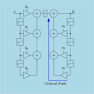

Verilog Code of Different IIR Low Pass Filters

IIR filters are very important in designing any signal processing or communication systems. Thus FPGA implementation of IIR filters must be known. Here, different structures of IIR low pass filters are implemented. Verilog code of each structure is provided here.

$4.00

Shop now

-1