Linear System Solvers - Digital System Design

1. Introduction

Solving systems of linear equations is a fundamental computational task in engineering, scientific computing, signal processing, control systems, and artificial intelligence. A general linear system can be represented as

$A\mathbf{x}=\mathbf{b}$

where ( $A\in\mathbb{R}^{n\times n}$ ) is the coefficient matrix, ( $\mathbf{x}\in\mathbb{R}^{n}$ ) is the unknown vector, and ( $\mathbf{b}\in\mathbb{R}^{n})$ is the known input vector.

The objective is to determine the unknown vector (\mathbf{x}) efficiently and accurately. The choice of solution technique depends on matrix properties, system dimensions, sparsity, numerical accuracy, computational complexity, and available hardware resources.

Efficient linear-system solvers are particularly important in hardware acceleration, where computational latency, throughput, power consumption, and resource utilization directly affect system performance.

2. Importance of Solving Linear Systems

Linear-system solvers are widely used in several computational applications:

Digital Signal Processing: Adaptive filtering, channel estimation, beamforming, and equalization.
Control Systems: State estimation, model predictive control, and system identification.
Machine Learning: Linear regression, optimization, parameter estimation, and neural-network computations.
Computer Vision: Image reconstruction, feature estimation, and geometric transformations.
Communication Systems: MIMO detection, channel estimation, and signal recovery.
Scientific Computing: Numerical simulation, finite-element analysis, and differential-equation solving.
Robotics: Localization, trajectory estimation, and sensor fusion.

The increasing computational demands of these applications have motivated the development of algorithms suitable for parallel processing and dedicated hardware implementation.

3. Categories of Linear-System Solution Techniques

Linear-system solution techniques can be broadly classified into the following categories.

3.1 Direct Methods

Direct methods obtain a solution through a finite sequence of arithmetic operations, subject to numerical precision and non-singularity conditions.

Common algorithms include:

Gaussian Elimination
Gaussian Elimination with Partial Pivoting
Gaussian Elimination with Complete Pivoting
Gauss–Jordan Elimination
LU Decomposition
Doolittle Decomposition
Crout Decomposition
Cholesky Decomposition
LDL(^T) Decomposition
QR Decomposition
Householder Transformation
Givens Rotation
Modified Gram–Schmidt Orthogonalization
Forward Substitution
Backward Substitution
Block LU Decomposition
Block Cholesky Decomposition

For example, LU decomposition expresses the coefficient matrix as

$A=LU$

where (L) and (U) are lower and upper triangular matrices, respectively. The solution is then obtained through forward and backward substitution.

3.2 Iterative Methods

Iterative methods generate successive approximations to the solution. They are particularly useful for large-scale and sparse systems.

Common algorithms include:

Jacobi Method
Block Jacobi Method
Gauss–Seidel Method
Successive Over-Relaxation (SOR)
Symmetric Successive Over-Relaxation (SSOR)
Richardson Iteration
Steepest Descent Method
Conjugate Gradient (CG)
Preconditioned Conjugate Gradient (PCG)
Biconjugate Gradient (BiCG)
Biconjugate Gradient Stabilized (BiCGSTAB)
Generalized Minimal Residual (GMRES)
Flexible GMRES (FGMRES)
Minimum Residual Method (MINRES)
Conjugate Residual (CR) Method
Chebyshev Iteration

The Conjugate Gradient method is particularly useful for symmetric positive-definite systems, whereas GMRES and BiCGSTAB are commonly applied to nonsymmetric systems.

3.3 Matrix Inversion Techniques

An alternative approach to solving a linear system is to calculate the inverse of the coefficient matrix, provided that the matrix is nonsingular.

The solution can then be expressed as

$\mathbf{x}=A^{-1}\mathbf{b}$

Common matrix inversion techniques include:

Gauss–Jordan Matrix Inversion
Adjugate and Cofactor Method
LU-Based Matrix Inversion
Cholesky-Based Matrix Inversion
QR-Based Matrix Inversion
Lower Triangular Matrix Inversion
Upper Triangular Matrix Inversion
Block Matrix Inversion
Schur Complement-Based Inversion
Newton–Schulz Iterative Matrix Inversion
Moore–Penrose Pseudoinverse

Triangular matrix inversion is particularly relevant to hardware implementations because triangular matrices frequently arise from LU and Cholesky factorization.

However, explicitly computing ( $A^{-1}$ ) is not always computationally efficient. When only the solution vector is required, direct or iterative solution methods are generally preferable.

3.4 Sparse and Structured Matrix Methods

Many engineering applications produce sparse or structured matrices. Specialized algorithms exploit these properties to reduce computational complexity and memory requirements.

Common techniques include:

Thomas Algorithm for Tridiagonal Systems
Cyclic Reduction
Parallel Cyclic Reduction (PCR)
Sparse Gaussian Elimination
Sparse LU Decomposition
Sparse Cholesky Decomposition
Banded Matrix Solvers
Block Tridiagonal Solvers
Block Cyclic Reduction
Multigrid Methods
Algebraic Multigrid (AMG)
Domain Decomposition Methods
Schur Complement Methods

These techniques are particularly useful in parallel computing architectures and hardware accelerators.

3.5 Least-Squares and Estimation Methods

When a system is overdetermined, underdetermined, or affected by measurement noise, least-squares techniques are often used to estimate the unknown variables.

Common methods include:

Normal Equation Method
QR-Based Least-Squares Solution
SVD-Based Least-Squares Solution
Weighted Least Squares
Total Least Squares
Tikhonov Regularization
Ridge Regression
Minimum-Norm Solution
Pseudoinverse-Based Solution

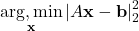
The least-squares problem is commonly represented as

$\underset{\mathbf{x}}{\operatorname{arg,min}}\left|A\mathbf{x}-\mathbf{b}\right|_2^2$

3.6 Optimization and Machine-Learning-Based Techniques

Optimization algorithms are closely related to linear-system computations and are widely used in machine learning and numerical optimization.

Representative techniques include:

Gradient Descent
Steepest Descent
Newton’s Method
Quasi-Newton Methods
Gauss–Newton Method
Levenberg–Marquardt Algorithm
Conjugate Gradient Optimization
Coordinate Descent
Neural-Network-Based Linear Solvers
Learned Iterative Solvers
Data-Driven Preconditioning
Physics-Informed Neural Networks (PINNs)

Backpropagation is also relevant to this category. It is not itself a linear-system solver; rather, it computes gradients through neural-network layers using matrix-vector and matrix-matrix operations. These computations are important in neural-network training and hardware acceleration.

4. Algorithms Relevant to Hardware Implementation

Not all numerical algorithms are equally suitable for hardware acceleration. The following techniques are particularly relevant to FPGA, ASIC, GPU, and DSP implementations.

Algorithm	Hardware relevance
Gaussian Elimination	Suitable for pipelined arithmetic architectures
LU Decomposition	Reusable factorization for multiple right-hand sides
Cholesky Decomposition	Efficient for symmetric positive-definite matrices
QR Decomposition	Useful for numerically stable least-squares computation
Givens Rotation	Suitable for iterative and pipelined architectures
Jacobi Method	Offers substantial parallelism
Conjugate Gradient	Useful for large sparse systems
Thomas Algorithm	Efficient for tridiagonal systems
Parallel Cyclic Reduction	Suitable for parallel hardware architectures
Triangular Matrix Inversion	Useful when the inverse is reused
Forward/Backward Substitution	Efficient triangular-system solution
Newton–Schulz Method	Matrix-multiplication-oriented inverse computation

5. Hardware Design Considerations

The selection and implementation of a linear-system solver in hardware depend on several important factors:

Parallelism: Availability of independent arithmetic operations for concurrent execution.
Pipelining: Ability to improve throughput through overlapping computational stages.
Resource Utilization: Number of LUTs, flip-flops, DSP blocks, and memory resources required.
Latency: Number of clock cycles required to obtain the solution.
Throughput: Number of systems or solutions processed per unit time.
Numerical Precision: Selection of fixed-point or floating-point arithmetic.
Arithmetic Complexity: Cost of multiplication, division, square-root, and accumulation operations.
Memory Requirements: Storage of matrices, intermediate results, and coefficients.
Power Consumption: Energy required for computation and data movement.
Numerical Stability: Sensitivity of the algorithm to finite-precision arithmetic and rounding errors.

For FPGA and ASIC implementations, algorithms that expose parallelism, support pipelining, and minimize memory and arithmetic overhead are often preferred.

6. Conclusion

Solving linear systems is an essential operation across signal processing, control engineering, communication systems, scientific computing, and artificial intelligence. Several approaches are available, including direct methods, iterative methods, matrix inversion, sparse matrix techniques, and least-squares algorithms. For hardware acceleration, the choice of algorithm must consider computational complexity, parallelism, memory requirements, numerical accuracy, latency, throughput, and power consumption. Algorithms such as LU decomposition, Cholesky decomposition, QR decomposition, Jacobi iteration, Conjugate Gradient, cyclic reduction, and triangular-system solvers provide useful foundations for FPGA, ASIC, GPU, and DSP implementations. The development of resource-efficient and high-throughput linear-system solvers remains an important research direction for real-time embedded systems and hardware-accelerated computing.